프로젝트: 판매 대시보드 만들기
선, 막대, 히스토그램, 주석, 스타일을 조합해 2 × 2 판매 대시보드를 만듭니다.
소개
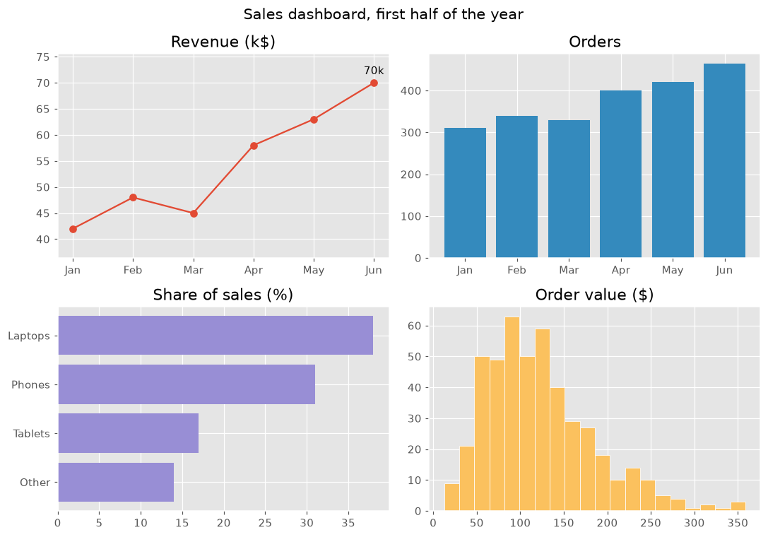
이 프로젝트는 강의 전체를 하나로 묶습니다. 한 그림에 네 개의 차트를 두고, 각각 같은 판매 데이터에 대한 질문 하나에 답합니다. 통일된 스타일과 명확한 제목 덕분에 대시보드를 한눈에 읽을 수 있습니다.
plt.style.use는 그림 전체의 색과 글꼴을 정합니다. 각 패널은 질문 하나에 답합니다. 매출은 어떻게 늘었는가(최고의 달에 주석을 단 선), 주문은 몇 건인가(막대), 무엇이 팔리는가(정렬한 가로 막대), 주문 금액은 보통 얼마인가(히스토그램). color="C1"은 스타일의 두 번째 색을 골라 패널마다 색을 다르게 하고, margins는 레이블 자리를 남깁니다. suptitle은 그림 전체 제목이고 tight_layout은 패널이 겹치지 않게 합니다. "fivethirtyeight"나 "bmh" 같은 다른 스타일도 써 보세요.
인터랙티브 시각화
스타일을 바꾸면 대시보드 전체 모양이 한 번에 바뀝니다. 패널을 고르면 그 패널을 그리는 코드를 볼 수 있습니다.
실행 가능한 Matplotlib 예제
Matplotlib
main.py
import matplotlib.pyplot as plt
import numpy as np

plt.style.use("ggplot")
months = ["Jan", "Feb", "Mar", "Apr", "May", "Jun"]
revenue = np.array([42, 48, 45, 58, 63, 70])
orders = np.array([310, 340, 330, 400, 420, 465])
products = {"Other": 14, "Tablets": 17, "Phones": 31, "Laptops": 38}
order_values = np.random.default_rng(8).gamma(4, 30, 465)

fig, axes = plt.subplots(2, 2, figsize=(10, 7))
fig.suptitle("Sales dashboard, first half of the year", fontsize=14)

axes[0, 0].plot(months, revenue, marker="o")
best = revenue.argmax()
axes[0, 0].annotate(f"{revenue[best]}k", (best, revenue[best]), xytext=(0, 8), textcoords="offset points", ha="center")
axes[0, 0].margins(y=0.2)
axes[0, 0].set_title("Revenue (k$)")

axes[0, 1].bar(months, orders, color="C1")
axes[0, 1].set_title("Orders")

axes[1, 0].barh(list(products), list(products.values()), color="C2")
axes[1, 0].set_title("Share of sales (%)")

axes[1, 1].hist(order_values, bins=20, color="C4", edgecolor="white")
axes[1, 1].set_title("Order value ($)")

fig.tight_layout()
plt.show()