プロジェクト: 売上ダッシュボード
折れ線、棒、ヒストグラム、注釈、スタイルを組み合わせて 2 × 2 の売上ダッシュボードを作ります。
はじめに
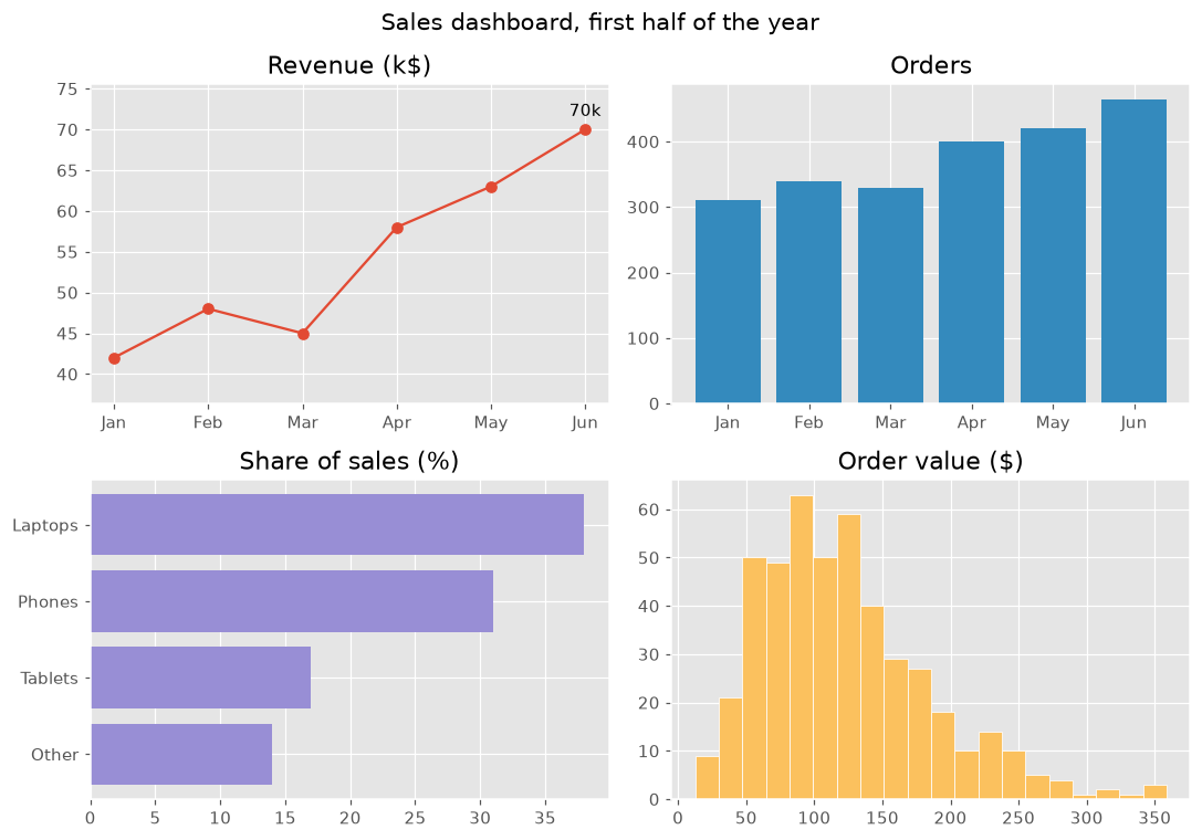
このプロジェクトではコースの内容をまとめます。1つの図に4つのグラフを置き、それぞれが同じ売上データについて1つの問いに答えます。統一したスタイルとわかりやすいタイトルで、ひと目で読めるダッシュボードになります。
plt.style.use は図全体の色とフォントを決めます。各パネルは1つの問いに答えます。売上はどう伸びたか (最高の月に注釈を付けた折れ線)、注文は何件あったか (棒)、何が売れているか (並べ替えた横棒)、注文金額はふつうどれくらいか (ヒストグラム) です。color="C1" はスタイルの2番目の色を選んでパネルごとに色を変え、margins はラベルの余白を作ります。suptitle は図全体のタイトル、tight_layout はパネルの重なりを防ぎます。"fivethirtyeight" や "bmh" など別のスタイルも試してみましょう。
インタラクティブ ビジュアライザー
スタイルを変えるとダッシュボード全体の見た目が一度に変わります。パネルを選ぶと、それを描くコードがわかります。
実行できる Matplotlib の例
Matplotlib
main.py
import matplotlib.pyplot as plt
import numpy as np

plt.style.use("ggplot")
months = ["Jan", "Feb", "Mar", "Apr", "May", "Jun"]
revenue = np.array([42, 48, 45, 58, 63, 70])
orders = np.array([310, 340, 330, 400, 420, 465])
products = {"Other": 14, "Tablets": 17, "Phones": 31, "Laptops": 38}
order_values = np.random.default_rng(8).gamma(4, 30, 465)

fig, axes = plt.subplots(2, 2, figsize=(10, 7))
fig.suptitle("Sales dashboard, first half of the year", fontsize=14)

axes[0, 0].plot(months, revenue, marker="o")
best = revenue.argmax()
axes[0, 0].annotate(f"{revenue[best]}k", (best, revenue[best]), xytext=(0, 8), textcoords="offset points", ha="center")
axes[0, 0].margins(y=0.2)
axes[0, 0].set_title("Revenue (k$)")

axes[0, 1].bar(months, orders, color="C1")
axes[0, 1].set_title("Orders")

axes[1, 0].barh(list(products), list(products.values()), color="C2")
axes[1, 0].set_title("Share of sales (%)")

axes[1, 1].hist(order_values, bins=20, color="C4", edgecolor="white")
axes[1, 1].set_title("Order value ($)")

fig.tight_layout()
plt.show()